Topological Data Analysis and Persistent Homology

The overall goal of Topological Data Analysis (TDA) is to be able to analyze topological features of data sets, often through computations of topological properties such as homology or via visualization. Here I will focus on the former technique, known as persistent homology, but I will briefly touch on the visualization aspect. Before jumping into the mathematical aspects I'll first give an overview of some motivations for TDA by both offering it as an alternative to typical statistical tools as well as showing some of the unique capabilities of TDA.

Motivations for Understanding Topological Properties of Data

In many sciences and other fields involving data collection and analysis, one can often consider two types of data analysis: qualitative and quantitative. Given a large and potentially complex data set \(D\), the task of qualitative data analysis is to investigate if \(D\) contains information you are looking for, and this is often performed via some type of visualization. If you then feel that \(D\) does contain desired information, then you can often proceed to applying a more quantitative technique for extracting that information, guided by your intuition from the qualitative analysis. I claim that common statistical techniques are very useful for both tasks, but on more complex data sets currently emerging in today's sciences can be inadequate, and that a topological approach may help. Let's look at some specific examples of both qualitative and quantitative data analysis, and motivate why topological techniques might help.

Clustering and Dimensionality Reduction

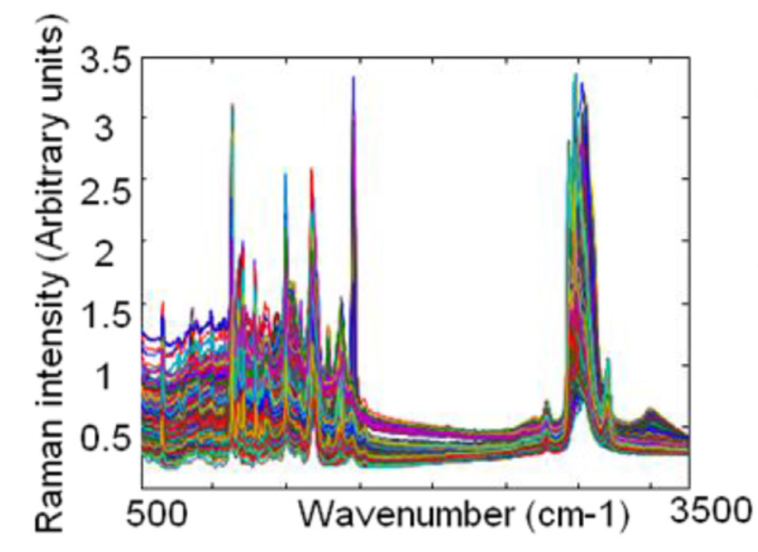
Consider an experiment in which we have a population consisting of multiple bacteria species¹, and we would like to determine how many different species are present. To do so we can use a technique called Raman spectroscopy, which in summary shines a laser into your sample and records a emission spectra of the sample. In this paper 4 species with 1000 bacteria each were tested with Raman spectroscopy (giving 4000 spectra) with each spectra consisting of 1500 intensity measurements for wavelengths between 500 and 3500 \(cm^{-1}\). Mathematically this gives us 4000 points living in \(\R^{1500}\). Now we want to see if the spectra can actually be used to differentiate the 4 bacteria species. Unfortunately, visualization of \(\R^{1500}\) directly is not helpful, as the following plot of overlapping spectra shows:

A very standard technique for reducing this high dimensional data down to a smaller dimension is PCA (Principle Components Analysis) which finds the linear projection which maximizes the variance. Using PCA to project \(\R^{1500}\) to \(\R^2\) gives the following plot, with colors indicating the previously known species:

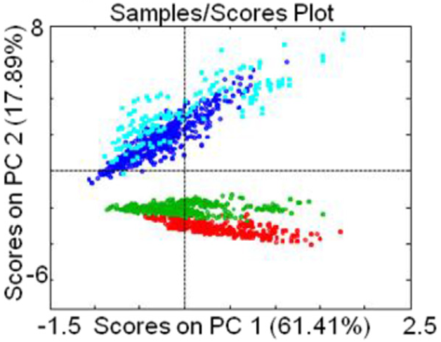
PCA has provided some useful information, but not so much as we would like. This linear projection shows that some differentiation of species using the spectra is possible, but unfortunately PCA can not be used to differentiate the blue and light blue samples as they strongly overlap. Any typical algorithm used to identify clusters (such as k-means clustering) would fail to isolate 4 clusters. The original data in \(\R^{1500}\) probably contains the information necessary to differentiate all 4 species, but we can't visualize it well directly. On the other hand linearly projecting to a low dimension destroys the useful information we want. Projecting to a higher dimensional space like \(\R^3\) or using non-linear dimensionality reductions such as t-SNE ² or diffusion maps ³ might or might not work better, but at the end of the day can run into the same limitations. Using topology we can take a different approach: imagine we can regard the data as a manifold \(X \subseteq \R^{1500}\); then detecting the number of different species (clusters) corresponds to determining the number of connected components of \(X\). Using TDA techniques we can determine the number of connected components in the original data set, without having to project to lower-dimensions. This type of clustering analysis is applicable to a huge number of problems, not just in the biological domain.

Understanding Higher-Dimensional Topological Features of Primary Visual Cortex of Monkeys

However, TDA can be used for more than just inspecting connected components. One particularly interesting application of TDA to neuroscience is discussed in section 2.5 of Carlsson ⁴. In an experiment a 10x10 array of electrodes were implanted in the Primary Visual Cortex of Macaque monkeys, while the monkeys viewed either a blank screen or some movie clips. A bunch of signal processing techniques were applied to the voltage sequences, eventually resulting in a collection of data sets, each consisting of 200 data points lying in \(\R^5\). Each such data set \(D_i \subseteq \R^5\) corresponds to the monkey looking at either a blank screen or movie clips, for a 10 second window. Each point \(p \in D_i \subseteq \R^5\) are the 5 voltages during a 50ms window of the top 5 activated neurons in the 10 second window associated to \(D_i\). So we have many such \(D_i \subseteq \R^5\), of which some correspond to watching blank screens and others correspond to watching movie clips.

The task now is to differentiate the \(D_i\)'s based on blank screen vs. movie clips. Given some \(D_i\), if we can view \(D_i\) as a topological space, then we can apply the algebraic topology tool of homology to compute the Betti numbers of \(D_i\). In this study the first 3 Betti numbers \((\beta_0, \beta_1, \beta_2)\) were computed for each \(D_i\). By a vast margin the most common Betti numbers were \(a = (1, 1, 0)\) and \(b = (1, 0, 1)\), corresponding to the topology of a circle and a sphere. Finally Betti numbers were computed for data sets generated by random firings according a Poisson model (i.e. the null hypothesis). The distribution of Betti numbers is easily able to distinguish all three modes (blank screen, movie clips, random Poisson model) from each other. In addition since \(a\) and \(b\) were the most common Betti numbers for both blank screen and movie clip modes, this suggests that the primary visual cortex seems to naturally operate using the topology of circles and spheres, but the reason for this topological phenomenon is not yet known.

Point Clouds and Simplicial Complexes

In both of the examples above and in nearly all data analysis settings one has a discrete finite data set \(D\). Often \(D \subseteq \R^n\), but more generally we consider \(D\) to be some discrete finite metric space (for example in comparing DNA sequences one can define a distance metric between sequences which is non-Euclidean). \(D\) is often called a point cloud. One way to look at this is that the point cloud \(D\) is drawn from a probability distribution with support some metric space \(X\). For example in the bacteria species classification experiment \(X\) would be the space of possible emission spectra for the 4 different species, and we would expect \(X\) to have 4 connected components. Thus the goal of TDA is to infer the topological properties of \(X\) given a point cloud \(D\) sampled from \(X\).

Since \(D\) is a discrete space, it is useless topologically as is. The main strategy of TDA is to build a simplicial complex from \(D\) such that the topological properties of the simplicial complex are similar to those of \(X\). Of course this isn't always possible as it is contingent upon a sufficient number of samples.

Nerves of Open Covers and the Čech Complex

The first and most natural technique for building a simplicial complex based on some topological space \(X\) is based on an open cover \(\mathcal{U}\) of \(X\). If \(\mathcal{U} = \{U_i\}, i \in I\) is an open cover of \(X\) then the simplicial complex called the nerve of \(\mathcal{U}\), \(N(\mathcal{U})\), is defined to have vertex set \(I\), with a \(k-1\) simplex \(\{i_1, \cdots, i_k\} \in N(\mathcal{U})\) if and only if: \[ U_{i_1} \cap U_{i_2} \cap \cdots \cap U_{i_k} \neq \emptyset \]

The following picture from Wikipedia illustrates this well:

Note that if at most \(n\) open sets intersect simultaneously then \(N(\mathcal{U})\) has dimension \(n-1\). A basic result of nerves is the Nerve Lemma:

We can now define the Čech Complex of a finite point cloud \(D \subseteq X\). Let \(\varepsilon > 0\), and define the open cover \(\mathcal{U} = \{ B_\varepsilon (x) \mid x \in D \} \). Then the Čech Complex of radius \(\varepsilon\) is defined as \(\check{C}_\varepsilon(D) = N(\mathcal{U})\).

Homotopy Type of the Čech Complex

To better understand the topological properties of the Čech Complex we can apply the Nerve Lemma. By the Nerve Lemma, \(\check{C}_\varepsilon(D) \homt \bigcup_{x \in D} B_\varepsilon(x)\). However, what we would like is to relate the topology of \(\C_\e(D)\) to the topology of \(X\), where \(D\) has been sampled from \(X\). The following theorem⁴ is a partial result in this direction:

1. Since we only have access to \(D\) and not \(X\), how can we know that \(X\) is a Riemannian manifold?
2. The existence of such an \(e\) is good, but the theorem offers no way to find or search for \(e\).
3. The largest issue is that we only have one given point cloud \(D\), so the existence of another \(D'\) guaranteeing homotopy equivalence is not useful.

There have been further results that partially address some of these issues, of which Chazal⁵ surveys a few. An additional problem with Čech Complexes is that computationally they are quite slow to compute, which leads us to consider alternate simplicial complex constructions such as the Vietoris-Rips Complex and many others which are surveyed by Carlsson⁴. However, the simplicial complex constructions are all similar in that they all attempt to reconstruct the homotopy type of \(X\) and can do so under strict assumptions, but in practical data analysis situations will almost always fail to be homotopy equivalent.

Exploring Some Čech Complexes

To get a better intuition for why Čech Complexes of point clouds \(D\) sampled from a topological space \(X\) fail to be homotopy equivalent to \(X\), we can look at visualizations of Čech Complexes on sample data sets. Since Čech Complexes can be quite high dimensional, we only visualize the 2-skeleton of the Čech Complex. Below you can interact with a variety of sample data sets, and vary the parameter \(\varepsilon\) to see how it affects \(\C_\e(D)^{(2)}\).

The above code was based on Wattenberg, et al.⁶. Play around with the Čech Complex visualization as long as you want. But once you're done, here are some of the key takeaways from it.

First, due to random sampling noise and non-homogenous density it can be tricky to chose a value of \(\e\) such that \(\C_\e(D) \homt X\). For example with the annulus you have to pick some \(\e\) that is large enough to fill in some holes from noise, but if you pick an \(\e\) that is way too big then it will fill in the hole of the annulus itself. For these toy data sets we can have an intuition for what choice of \(\e\) "looks right", but for high dimensional data it is hard to have an understanding of a "good" choice of \(\e\).

Second, there can be multiple "good" choices of \(\e\). For example, consider the 4th data set above with 2 circles of vastly different sizes. For \(\e \approx 0.07\) The tiny circle obtains the correct topology, but the big circle is still disconnected. But if you try to increase \(\e\) so as to make the big circle connected, the tiny circle actually becomes simply connected. Both the big and tiny circles have the homotopy type of a circle, but the homotopy type of each is only visible at distinct values of \(\e\). In a sense \(\e\) is like the amount of zoom in a microscope: you can make \(\e\) very small to zoom in closely and inspect the topology of the tiny circle, or you can make \(\e\) large to zoom out and observe the topology of the big circle, at which point the tiny circle is negligible.

The second point really provides the key insight of TDA: There is no one best value of \(\e\), but rather the spectrum of topologies as \(\e\) varies provides a comprehensive view of the topology of the point cloud. This will also address the first point, as the holes due to noisy sampling only last for a short range of \(\e\) values. Thus, in TDA we study families of simplicial complexes such as \(\P = \{\C_\e(D) \mid \e \in T \subseteq \R \}\). The crucial property of these Čech Complex families is that for \(\e \leq \e'\) we have that \(\C_\e(D)\) is a subcomplex of \(\C_{\e'}(D)\) (this is a trivial result of the definition of a Čech Complex). Also note that since point clouds are finite, only finitely many \(\e\) will produce distinct Čech Complexes, so we can consider \(T\) to be finite. Other simplicial complex constructions such as Vietoris-Rips complexes also share these properties.

Persistence

Persistence Objects

We briefly set aside the specific construction of Čech Complexes and work from an algebraic perspective. Let \((T, \leq)\) be any partially ordered set and let \(\underline{C}\) be any category. We say that a \(T\)-persistence object is a family \( \{c_t\}_{t \in T} \subseteq \underline{C} \) together with a morphism \(\phi^{t,u} : c_t \to c_u \) whenever \(t \leq u\) such that if \(t \leq u \leq v\) then \(\phi^{u,v} \circ \phi^{t,u} = \phi^{t,v}\). Alternatively a \(T\)-persistence object can be viewed as a functor \(\Phi : T \to \underline{C}\). Diagrammatically this looks something like:

Suppose we have a \(T\)-persistence object \( \{c_t, \phi^{t,u} \} \) and some partial order preserving map \(f : T' \to T\) for some other partially ordered set \(T'\). Then we have an induced \(T'\)-persistence object \( \{c_{f(t')} \}_{t' \in T'} \) with morphisms \(\psi^{t',u'} : c_{f(t')} \to c_{f(u')}\) given by \(\psi^{t',u'} = \phi^{f(t'),f(u')}\). It sounds more complicated than it is, so hopefully a diagram clarifies:

Čech Complex families as Persistence Objects

We can easily see that Čech Complex families are \(\R\)-persistence simplicial complexes since for all \(\e \leq \e'\) we have the inclusion map \(i^{\e,\e'}: \C_\e(D) \hookrightarrow \C_{\e'}(D)\) as discussed above (the superscript notation denotes Čech Complex radius, and is unrelated to cohomology). In addition since there are only finitely many values of \(\e\), say \(E = \{\e_1, \cdots, \e_n\} \subseteq \R\), which produce distinct Čech Complexes, we can easily construct an order preserving map \(f: \N \to E\), and thus we have that a Čech Complex family is an \(\N\)-persistence simplicial complex. For now we will work with \(\R\)-persistence, but will return to using \(\N\)-persistence later.

The inclusion maps \(i^{\e,\e'}: \C_\e(D) \hookrightarrow \C_{\e'}(D)\) for an \(\R\)-persistence simplicial complex then induce chain maps for the simplicial chain complex \( i_k^{\e,\e'}: C_k(\C_\e(D); G) \rightarrow C_k(\C_{\e'}(D); G) \), and likewise for the simplicial homology \( i_k^{\e,\e'}: H_k(\C_\e(D); G) \rightarrow H_k(\C_{\e'}(D); G) \) for any coefficient group \(G\). We can see this in a diagram, for \(\e \leq \e+p\):

To better understand what these inclusion induced maps are doing, we can look at a specific example from the visualization above. Consider two choices of \(\e\) for the annulus:

\(\C_\e(D)\)	\(\C_{\e+p}(D)\)

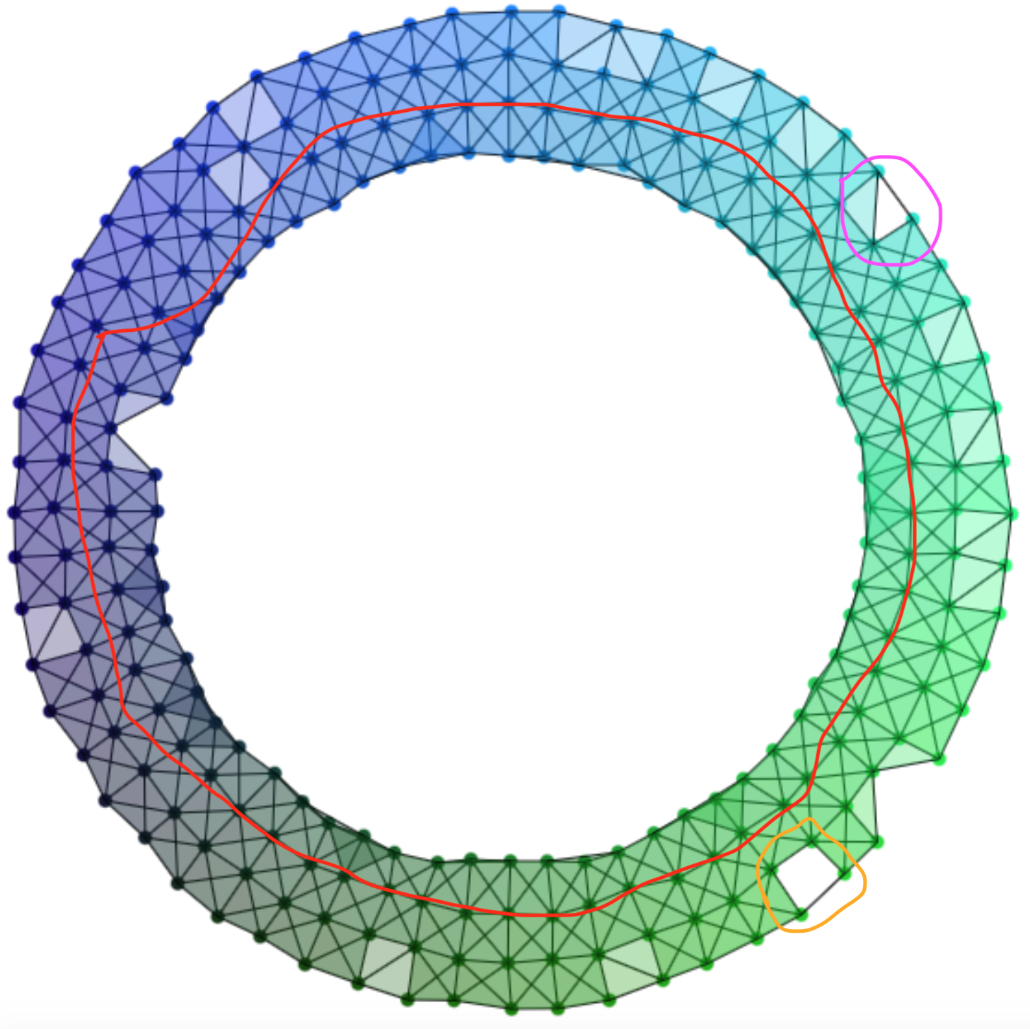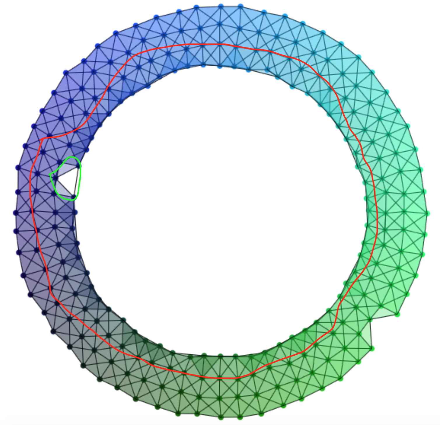In the left Čech Complex there are 3 generators for \(H_1\), shown in red, purple and orange. If we slightly increase \(\e\) to \(\e+p\) in the right Čech Complex we kill the purple and orange generators, but a new green generator is born. But if we look at the image of the homomorphism induced by the inclusion we see only that purple and orange are killed, leaving only the red generator in the image. In this case the inclusion induced homomorphism for \(\e\) to \(\e+p\) killed the topological features introduced by sampling noise, but whether or not this happens depends on the values of \(\e\) and \(p\). We define a new object called the \(p\)-persistent homology in order to capture the elements of \(H_k\) that survive an increase of the Čech Complex radius by \(p\). Formally, we define the level-\(k\) \(p\)-persistent homology group starting at radius \(\e\) to be: \[ H_k^{\e,\e+p}(\C_\e(D); G) := \Ima (\;i^{\e,\e+p} : H_k(\C_\e(D); G) \to H_k(\C_{\e+p}(D); G)\;) \] This is precisely the elements of the level-\(k\) homology of the Čech Complex with radius \(\e\) that are not killed by increasing the radius by \(p\). Note that this generalizes normal homology, as \(H_k^{\e,\e+0}(\C_\e(D); G) = H_k(\C_\e(D); G)\).

Graded Modules Correspondence

The \(p\)-persistent homology groups are what we would like to compute, but unfortunately the definition above does not offer a scheme for carrying out the computation. To remedy this we will develop a structure theorem for persistence. Let \(\mathcal{M}\) be an \(\N\)-persistence module over \(R\). Concretely we have a family of \(R\)-modules \(\{M^i\}_{i \in \N}\) with linear maps \(\phi^i : M^i \to M^{i+1}\) (this is sufficient to generate maps from \(M^i\) to \(M^j\) for \(i \leq j\)). Let \(R[t]\) with degree of \(t\) being 1 be the standard graded polynomial ring. We map \(\mathcal{M}\) to a graded module over \(R[t]\) as follows:

\[ \alpha(\mathcal{M}) := \bigoplus_{i=0}^\infty M^i \]

We say that the \(n\)-th graded part of \(\alpha(\mathcal{M})\) is \(M^i\). Lastly we need to describe scalar multiplication by the polynomial generator \(t\) on a vector \((m^0, m^1, m^2, \cdots)\) for \(m^i \in M^i\). We define this as: \[ t (m^0, m^1, m^2, \cdots) := (0, \phi^0(m^0), \phi^1(m^1), \phi^2(m^2), \cdots) \] The action of \(t\) is simply to shift each element up one gradation level by means of using the linear maps \(\phi^i\) provided by the persistence module. It is easy to check that \(\alpha\) defines a functor from the category of persistence modules over \(R\) to the category of graded

The intuition is that we use multiplication by \(t\) to keep track of the number of times an element of a module is mapped through the linear persistence maps.

Classification Theorem for \(\mathbb{N}\)-Persistence Modules

Showing that persistence modules are in correspondence with graded modules over \(R[t]\) opens the door to applying well-know classification theorems of graded modules. Unfortunately there is no simple classification when \(R\) is not a field, but for \(R = F\) a field, there exists a nice result:

There are two components to the classification. On the left side of \(\oplus\), we have the free part which corresponds to elements of the persistence module that appear at index \(i_s\) and never disappear. On the right side we have the torsion part which corresponds to elements of the persistence module that appear at index \(j_r\) and die at index \(j_r + l_r\). This classification is the main result we are looking for, since this gives us a concrete computational tool with which to calculate \(p\)-persistence homology groups. In particular the torsion part above corresponds precisely to the \(p\)-persistence homology groups discussed previously. Note that using \(R = F\) a field means that rather than having persistence modules, we have persistence vector spaces. But to be able to apply this theorem we need to know that our graded modules over \(F[t]\) are finitely generated. The following theorem provides an exact condition:

In light of this condition we can give our final conclusion on the classification of \(\N\)-persistence vector spaces by incorporating the intuition discussed above. For a field \(F\) and any \(0 \leq m \leq n\) we define an \(\N\)-persistence vector space \(\mathcal{U}(m, n) := \{U_i(m, n), \phi^i\}\) where \(U_i(m, n) = F\) for \(m \leq i \leq n\) and 0 otherwise, and \(phi^i\) is defined to be the identity function for \(m \leq i \leq n-1\) and the 0 function otherwise. In addition we allow \(n = \infty\). If \(\mathcal{V}\) is an \(\N\) persistent vector that satisfies the conditions in the above theorem, then we have the following classification result:

There is a quite nice and practical way to visualize this decomposition, called a persistence barcode. Each \(U(m, n)\) is drawn as a bar from index \(m\) to \(n\) with indices along the x-axis and different bars along the y-axis:

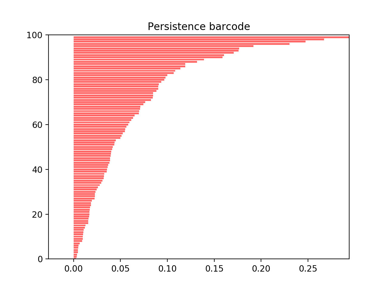
The start of a bar at \(m\) corresponds to the birth of a new \(U(m, n)\), until the bar disappears at index \(n\).

Applying Persistence Module Theory to Čech Complexes

Let's leave the area of abstract algebra and conclude by applying the results of persistence module classification to Čech Complexes. Recall that varying values of radii gives inclusion maps between Čech Complexes of increasing radius. These inclusion maps induce homomorphsims at the simplicial chain level and at the simplicial homology level, thus making \(H_k(\C_\e(D); R)\) an \(\R\)-persistence module over \(R\) with linear maps the homomorphisms induced by inclusion. In addition recall that since \(D\) is a finite point cloud only finitely many \(\e\) will produce distinct complexes, so we can enumerate these \(\e_i\)'s to consider \(H_k(\C_\e(D); R)\) an \(\N\)-persistence module over \(R\) with linear maps \(\phi^i = i_k^{\e_i,\e_{i+1}}\).

In order to apply the classification results we must choose \(R = F\) to be a field, such as \(\mathbb{Z}_2\), and then we have \(H_k(\C_\e(D); R)\) is an \(\N\)-persistence vector space over \(F\). In addition since \(D\) is finite each Čech Complex built from \(D\) will be finite and thus each \(H_k(\C_\e(D); F)\) will be finitely generated. Lastly, since we have only finitely many \(\e\), \(H_k(\C_\e(D); F)\) is tame. Therefore we can use the classification theorem above to compute persistent homology barcodes!

Future Directions of Persistent Homology

I've only outlined the most direct path for computing persistent homology from a point cloud. However, there are many other fascinating and important aspects to consider. In particular, studying the stability of persistent homology computations involves seeing if slightly altering the point cloud \(D\) will drastically affect the barcode result, while statistical approaches to persistent homology consider more carefully the underlying probility distribution from which a point cloud is sampled, thus turning a barcode into a probabilistic object. Chazal⁵ gives a survey of both of these directions of current research.

Using the GUDHI Python Library to Compute Persistent Homology

I would like to conclude on a matter of practicality. While understanding the underlying math is insightful and fun, I believe that TDA can have a significant impact on a wide number of fields and applications. Fortunately, algorithms to compute persistent homology have been implemented for Python in the GUDHI Library. Using computing persistent homology via GUDHI is quite easy, and I believe can offer interesting and new insights for fields with data analysis. I won't include a full tutorial, but a simple example of GUDHI in action should be sufficient to show how easy it is:

import gudhi as gd
import numpy as np
import matplotlib.pyplot as plt

def circle_sample(n, r):
    angles = np.random.uniform(0, 2*np.pi, n)
    return r*np.cos(angles), r*np.sin(angles)

# First we sample 150 points from the unit circle and the radius 2 circle
xs1, ys1 = circle_sample(150, 1.0)
xs2, ys2 = circle_sample(150, 2.0)
xs, ys = np.concatenate((xs1, xs2), axis=None), np.concatenate((ys1, ys2), axis=None)

# Then we build a Vietoris-Rips complex (2 skeleton)
pts = list(zip(xs, ys))
rc = gd.RipsComplex(points=pts, max_edge_length=4.1)
# Then we build a simplex tree, which is a fast data structure encoding the simplex
# This is just an intermediate step
tr = rc.create_simplex_tree(max_dimension=2)
# Finally we compute the persistence, which is a list of the form [(k, (b, d))]
# where k is the homology level, b is the birth time and d is the death time.
diag = tr.persistence()

# Then we plot the persistence barcode and the original data side by side.
plt.subplot(1, 3, 2)
gd.plot_persistence_barcode(diag)
plt.subplot(1, 3, 3)
gd.plot_persistence_diagram(diag)
plt.subplot(1, 3, 1)
plt.title("Original data set")
plt.plot(xs, ys, "ro")
plt.show()

Running this code produces the following plots:

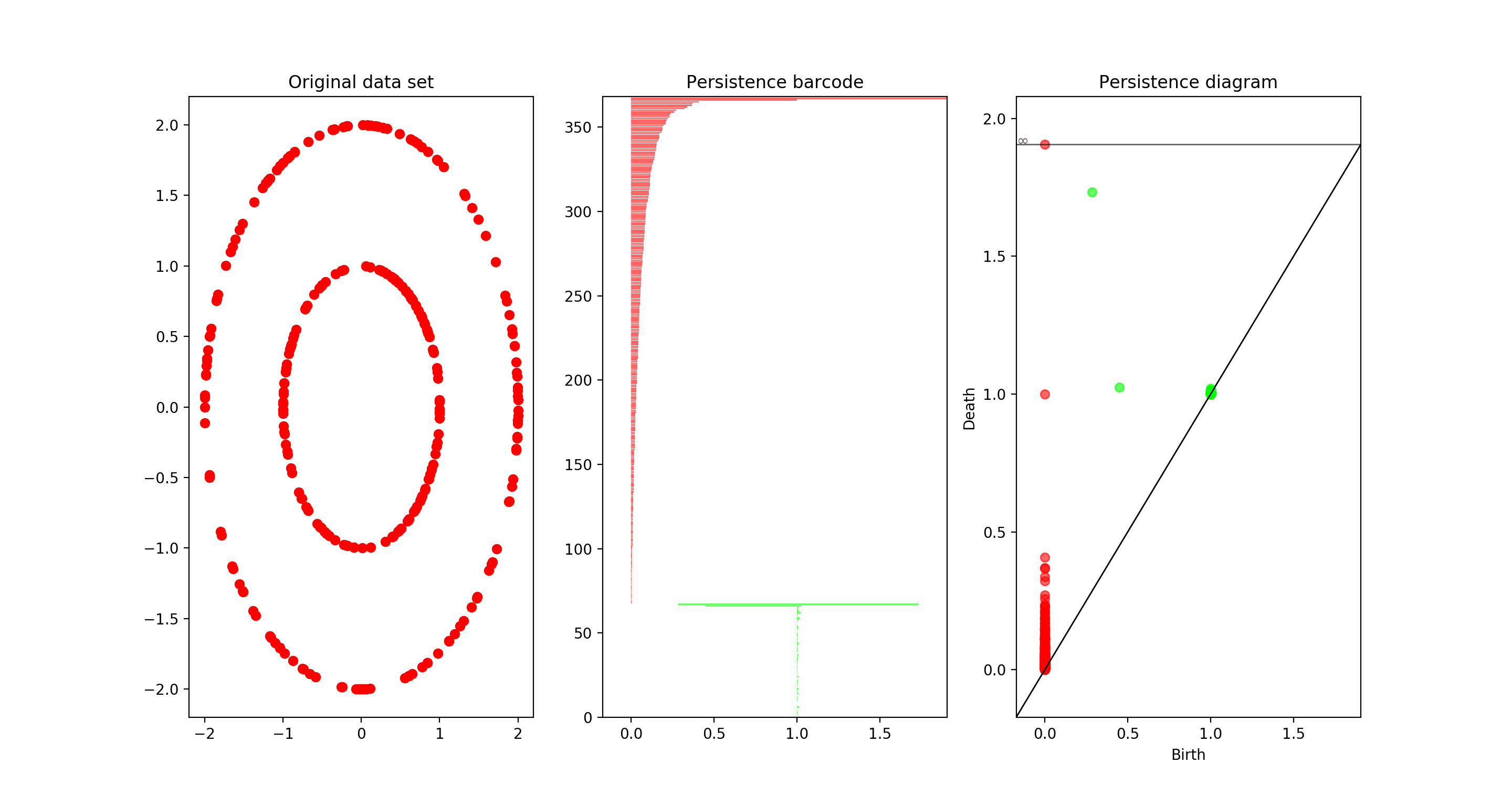
In particular it shows the correct computation of the Betti numbers \(\beta_0 = 2, \beta_1 = 2\).

References